Sampling Theorem

We all know that there are two kinds of signals:
1. Analog Signals
2. Digital Signals
We know that the signals that exists in nature are analog by default. And we also know that the signals that we store on our computers and memory devices like pen-drives, hard disks, SD cards and so on are of-course digital in nature.
Now the question that might come to your mind:

how do you convert an analog signal to a digital signal?

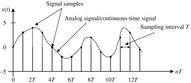
The answer to that is simple, first we sample the analog signal, and then we quantize it. Sampling is a process where in you hold the analog signal’s amplitude for a brief amount of time, so that the continuous time and continuous valued signal, becomes discrete time, continuous valued signal.

Now, there’s a theorem that governs the sampling process. Harry Nyquist, a Swedish electronic engineer came up with it. Now, it’s known as the sampling theorem.

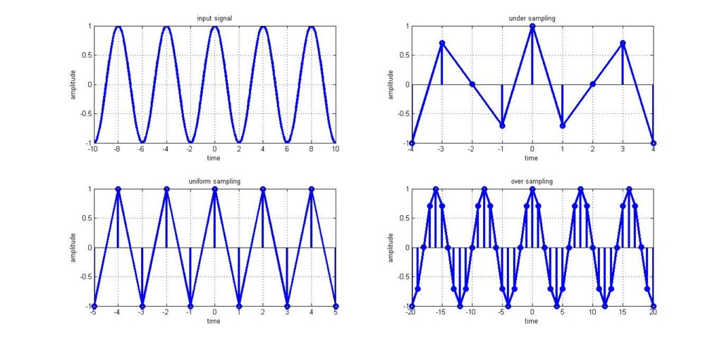
Sampling Theorem states that the minimum sampling rate for an analog signal, when uniformly sampled is two times that frequency of the analog signal being sampled. Or in simple words, the sampling frequency must be twice that of the signal being sampled.

$f_{s} >= 2f_{m}$

This minimum frequency, or the sampling rate is also called as the Nyquist rate.

Proving Sampling Theorem in MATLAB.

So basically, we need to prove that when a signal is sampled at a frequency less than the Nyquist Sampling rate, proper recovery of the signal is not possible. We can easily prove it in the frequency domain. When the sampling frequency is less than Nyquist Rate, we can show that the recovered signal’s frequency is not same as that of the actual analog signal.

MATLAB Code to prove Nyquist Sampling Theorem

You can download the complete code at the end of this post.

Before we start, we make sure that the workspace is cleaned.

clear all;
close all;
clc;

Next, we initialize all the required variables

widthOfTheLine = 1.5;
numberOfWaves = 5; % Number of waveforms to be shown
messageSignalFrequency = input("Enter the Message Signal Frequency: "); % Taking the user's input for Message Signal Frequency
initialSamplingFreq = 50*messageSignalFrequency; % Sampling Frequency for Unsampled Signal
timePerSample = 1/initialSamplingFreq; % Time needed for a single sample
stopTime = 1; % Samples to be generated up to.
timeAxis = 0:timePerSample:stopTime-timePerSample; % Generating the time axis
totalNumberOfSamples = size(timeAxis,2); % Calculating the number of samples
samplingFrequencyInterval = initialSamplingFreq/totalNumberOfSamples; % Calculating the frequency interval to generate the frequency axis;
frequencyAxis = -initialSamplingFreq/2:samplingFrequencyInterval:initialSamplingFreq/2-samplingFrequencyInterval; % Generating the Frequency Axis
phiDegrees = 90; % in degrees
phi = phiDegrees * pi / 180;

widthOfTheLine – It is the width of the line on the plot.
numberOfWaves – Number of waves of the signal to be shown on the plot.
messageSignalFrequency – Frequency of the signal to be sampled.
initialSamplingFreq – It is 50 times that of the message signal frequency, just to show the unsampled analog signal as smooth as possible.
stopTime – Samples will be generated up to stopTime.

We take a 90 degree phase shift so as to avoid the “0” sampled signal value for a perfectly sampled signal. You could easily replace the sin with a cos function and avoid adding the phase shift to the signal.

Check Out my other Posts

Pages: 1 2

Sampling theorem | Verification of NYQUIST’S sampling theorem using MATLAB

how do you convert an analog signal to a digital signal?